Network Demand Charges: How Tariff Complexity Affects the Flexibility Business Case
The Scale of the Opportunity
Network demand charges can be one of the biggest drivers of the flexibility business case.
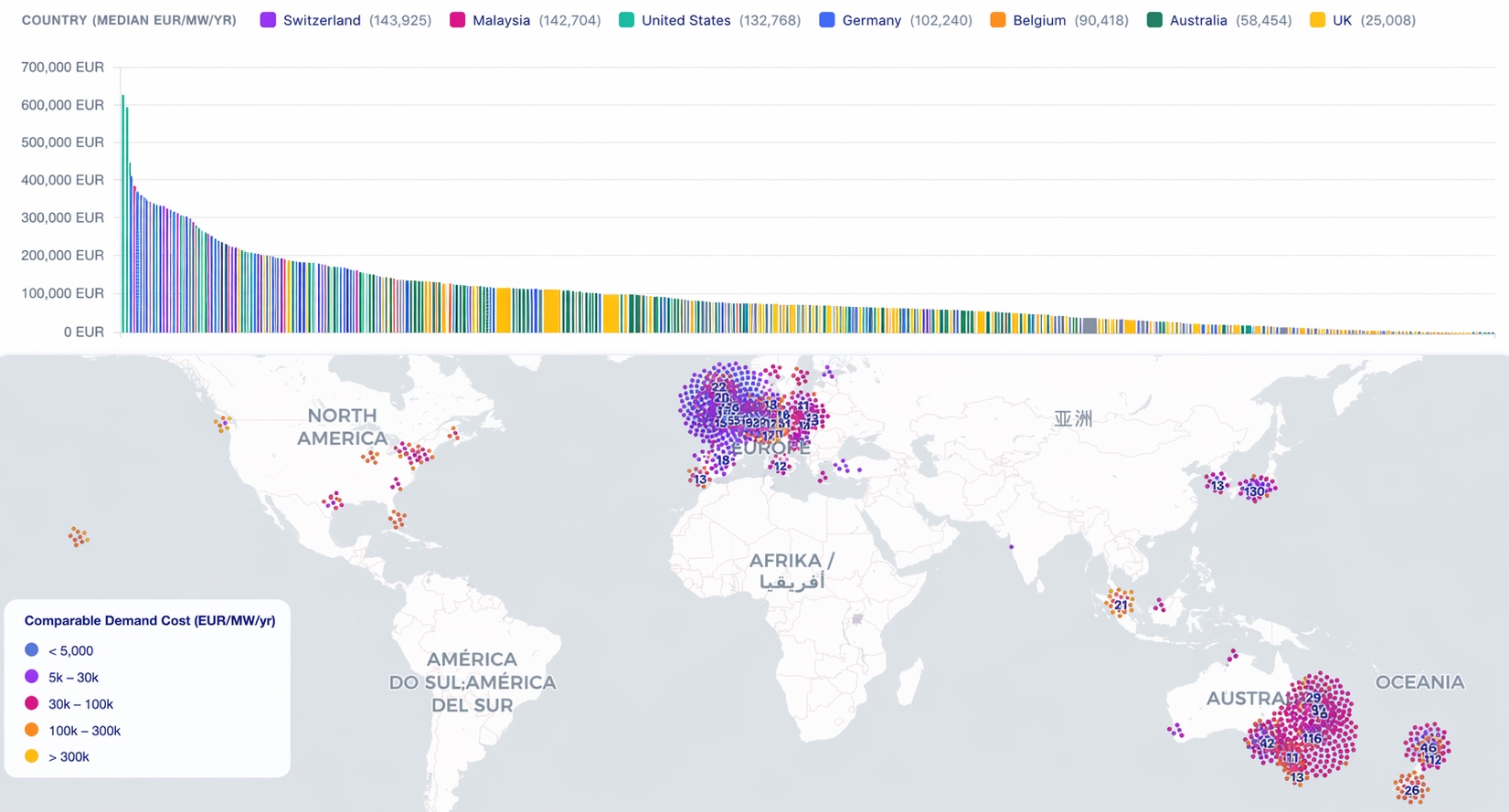
We looked at a selection of tariffs in the Gridcog Library that had some form of demand charge. Across 1,950 tariffs from 119 networks in 28 countries, the median annual demand charges for a 1MW load was about €47k/MW-year. The 90th percentile was about €159k/MW-year, and the upper end reached an eye-watering €624k/MW-year. The chart below shows a ranked list of tariffs by estimated demand cost, colour coded by country, and map highlighting the locations of some of the included networks.
Selection of tariffs with demand charges from the Gridcog Library
These tariffs aren’t exactly comparable because they apply to different kinds of loads or generation at different voltage levels in the transmission and distribution system, but this spread of commercial outcomes is reflective of the opportunity that can be available to large loads by using flexibility to manage peak demand.
But the story is not only about the size of the opportunity. It’s also about complexity of analysis.
What makes network demand charges challenging is that they are often much more than a single “$/kW/month” line item. They can depend on time-of-use windows, seasonal peak periods, contracted capacity, excess-demand penalties, annual utilisation thresholds, reactive power treatment, export treatment, bands, blocks, and more. Network operators can be very creative when defining the pricing arrangements for the use of the network.
For anyone trying to assess the value of flexibility, being able to handle that complexity matters just as much as the headline number.
Gridcog is built for exactly this problem. The challenge is not just representing tariff rates. It is accurately simulating and optimising the dispatch behaviour of flexible resources like battery storage systems that have to respond to these weird and wonderful pricing arrangements.
Some specific examples
Let’s dig into some specific examples to get a sense of the different kinds of tariff structures modelling of these projects needs to be able to handle.
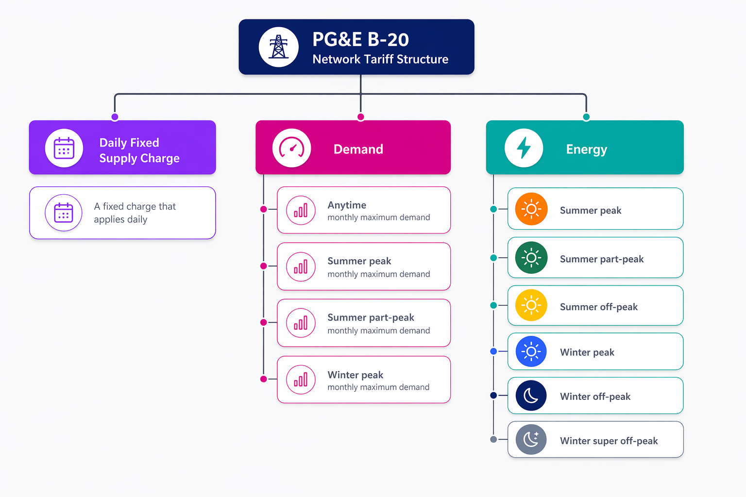
1. United States: PG&E B-20 Medium General Demand
This tariff has multiple demand charge components that stack on top of each other.
Indicative annual demand costs:€586k/MW/year
2. New Zealand: WEL Networks 655 Large Customers LV
This tariff has seasonal demand charges and with an excess demand charge that applies above a contracted fixed capacity with additional treatment for lower power factor.
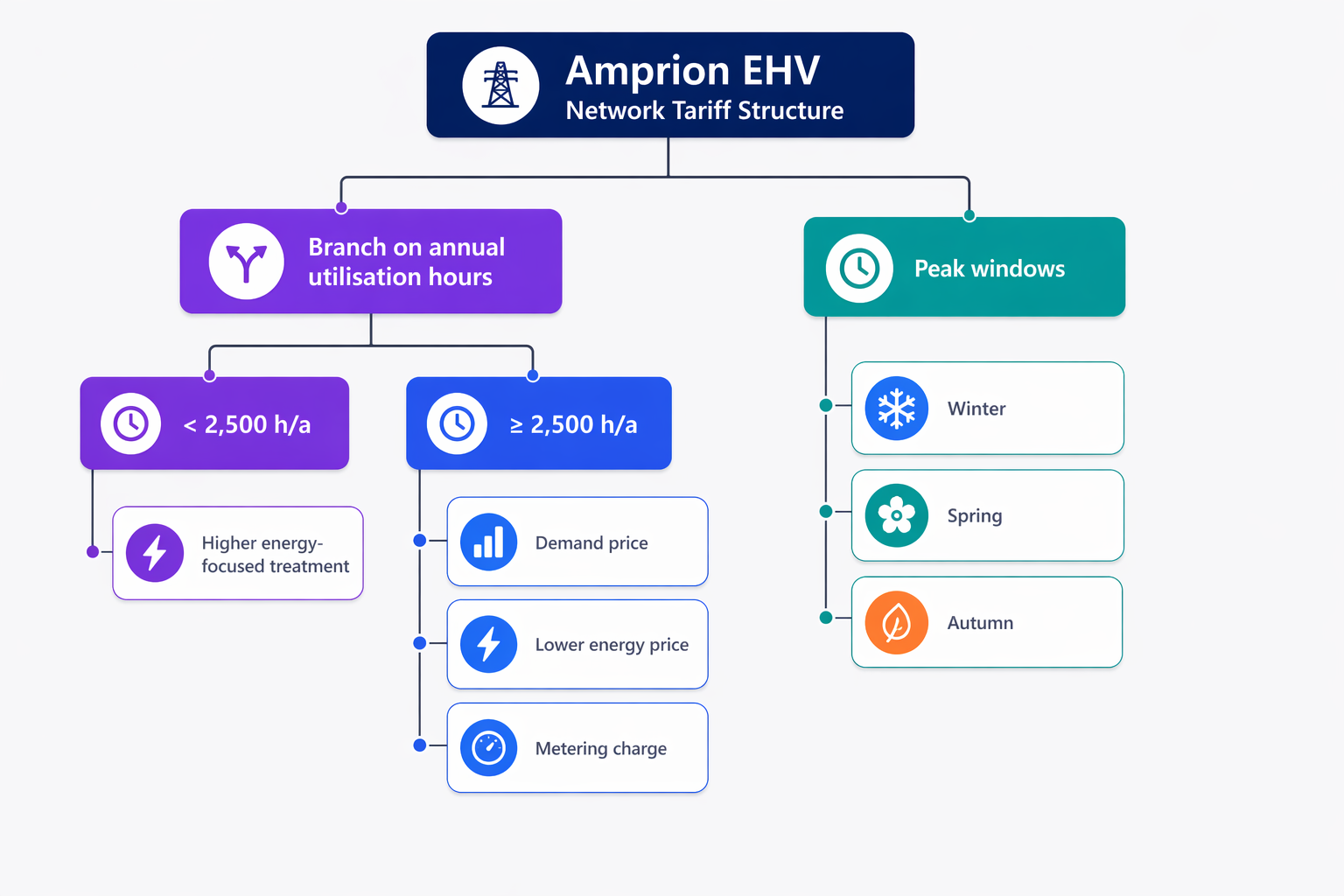
This tariff has a band structure where the pricing arrangement depends on “annual utilisation hours (Benutzungsstunden)”, which is a measure of the utilisation of the network calculated as annual energy withdrawn divided by annual peak demand.
Indicative annual demand costs: €53k/MW/year
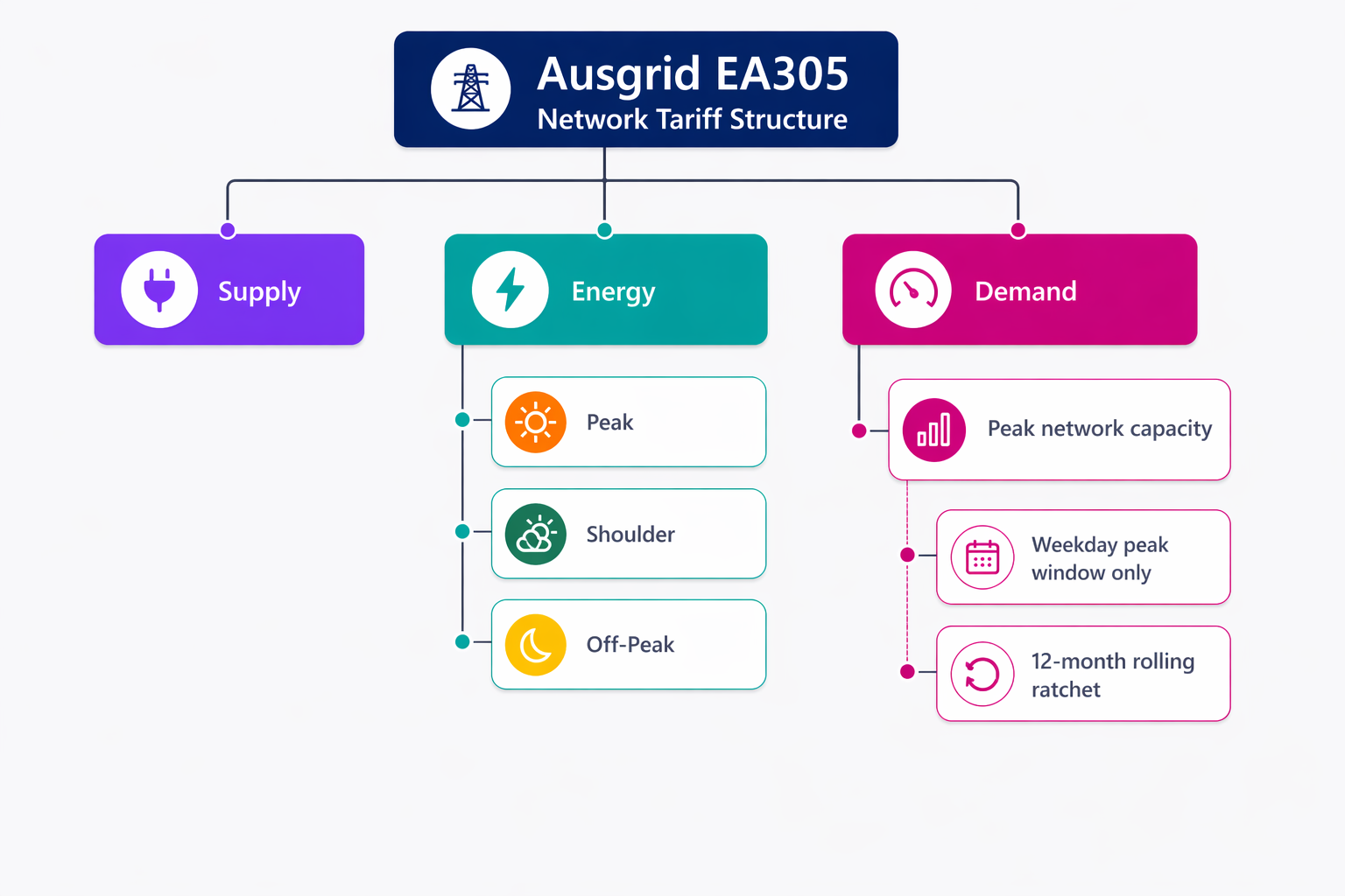
4. Australia: Ausgrid EA305
This tariff has a time-of-use based on demand charge on a 12-month rolling ratchet, which means if you exceed your previous maximum demand, even if only for 30-minutes, you will be incurring high network costs for the next 12-months.
Indicative annual demand costs: €144k/MW/year
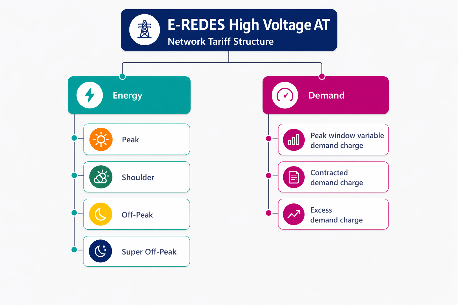
5. Portugal: E-REDES High Voltage AT
This tariff has contracted-capacity charge with a measured peak-window demand charge and an excess-demand treatment. It also layers a four-period seasonal energy time map on top.
Indicative annual demand costs: €58k/MW-year
So to model the flexibility business case properly, modelling needs to capture a lot more than energy time of use, and a simple, single maximum demand rate. Some of the key things to look for in your modelling solution are:
1. Layered time maps, precedence, and interval resolution
A tariff can define TOU periods at the tariff level or at the item level, with item-level time maps taking precedence. Time maps can be built from combinations of months, days, and hours, can overlap, and are applied in sequence so later definitions override earlier ones. They can also run at different resolutions, including half-hourly or quarter-hourly intervals. In practice, that means the model has to know exactly which intervals fall into which charging window for each line item.
2. Shared rate structures across energy, export, and demand
Energy, export, and demand items all use the same general item-rate structure. A tariff can apply a single flat rate, different rates by TOU, or threshold-based structures using blocks or bands. Those can be combined, so a tariff can be both TOU and block-based at the same time. That matters because flexibility value often sits in the interaction between time windows and thresholds, not just one or the other.
3. Multiple demand calculation types
Demand is not one thing. The engine needs to support kVA demand, kW demand, net demand, export demand, and minimum export demand. It also needs fixed demand constructs such as fixed kW, fixed kVA, fixed TOU kW, and fixed TOU kVA. A tariff can therefore charge on measured import, net load after generation, fixed contracted capacity, export peaks, or even minimum export over a window.
4. Demand windows, ratchets, resets, and averaging
Demand can be billed on the maximum in the current month, a rolling multi-month ratchet, a season that resets in a nominated month, or an averaged demand over a nominated number of intervals. Initial demand can also be carried in to model a site rolling off a previous high value. This is a major part of the flexibility business case because one event may affect one bill, or it may affect twelve.
5. Minimums, thresholds, and excess-demand rules
A tariff model needs to represent minimum billable demand, demand thresholds below which no charge applies, and explicit excess-demand treatment above a threshold or contracted value. These can be defined globally or by TOU, and they can also be pulled in as site-specific parameters. In practice, this is where contracted maximum demand, excess demand, and similar constructs live.
6. Blocks and bands on both energy and demand
Blocks and bands are not limited to energy. Demand items and export items can also be threshold-based, with daily, monthly, or quarterly block periods. A block structure applies different rates to different slices of usage. A band structure applies one rate to the whole quantity based on which band the site lands in. That distinction can materially change the marginal value of flexibility around a breakpoint.
7. Explicit export constructs
A modern tariff model needs to handle export as a first-class charging dimension. That includes flat export tariffs, blocked export, export demand charges, and peak export constructs. It also includes sign conventions, because import and export are not always treated symmetrically. For storage projects, it is increasingly common that export behaviour matters just as much as import behaviour.
8. Critical-interval and system-peak charging
Some tariffs are driven not by repeating TOU windows but by specific lists of intervals, such as system peaks, triads, IRCR, or critical peak demand events. These require the model to ingest raw peak intervals, apply the correct timezone and season reset date, and then aggregate demand or energy across those specific intervals using methods such as median, mean, or daily maximum. This is very different from ordinary monthly peak logic.
9. Reactive power and low power factor
Low-power-factor charges can be modelled either as an energy-style reactive charge or a demand-style reactive charge. They depend on a threshold for reactive energy or reactive demand relative to active consumption. For larger industrial sites, that can materially alter the economics of site control and network charges.
10. Future rates and future ratios
Tariffs do not stay static. The engine needs to be able to apply explicit future rates at specific dates, and also future ratios such as linear, compound, or annual percentage changes. This matters whenever the business case spans several years and the tariff is expected to escalate over time.
11. Loss factors and channel-specific billing
Some items need transmission or distribution loss factors applied multiplicatively. Others need to bill against a different channel altogether, such as a genset, EV charger, or a specific import or export flow. At the tariff level, channel maps can replace standard import or export with sums of custom channels. Without that, a model cannot correctly represent hybrid sites with multiple assets and flow paths.
12. Site-specific parameters and tariff updates
Many tariffs are templates until a site-specific value is inserted. Contracted demand, minimum billable demand, excess-demand thresholds, and fixed TOU demand can all be pulled from site specific tariff parameters. On top of that, scenarios or sites can apply tariff updates or tariff-item updates to override named values. That is important because a real project often uses one generic tariff with site-specific CMDs, export limits, or contract values layered on top.
In other words, the flexibility business case depends on modelling how a tariff is triggered, what quantity it measures, which intervals count, how long the effect persists, and which site-specific parameters sit behind it.
The takeaway
Network demand charges are both important and complicated.
That is precisely why they are such a strong use case for Gridcog. The commercial case for flexibility depends on getting these tariffs right, and getting them right requires more than a spreadsheet with a few rate inputs. It requires tariff data, tariff logic, and a simulation environment that can represent both.
As network tariffs become more conditional and more cost-reflective, that becomes even more important. The value of flexibility will increasingly depend not just on a site’s load profile, but on how well the underlying tariff mechanics are captured.
We explore how distribution networks can adapt to support renewable energy growth through flexible connections, local flexibility, and innovative tariffs.
.png)